A1 Bott (1969) 2D gravity algorithm

Two dimensional gravity anomalies are calculated using a python implementation of Bott’s (1969) [1] algorithm. This is similar to that derived by Talwani et al., (1959) [10] and operates by setting the observation point as the origin of a Cartesian coordinate system and treating the periphery of a given body as an n-sided polygon, defined by a discrete set of nodal points. The total gravity anomaly is then calculated by evaluating the solution for a semi-infinite horizontal slab with one sloping interface for each set of nodal pairs and then summing the results. The analytic solution for this is given by Heiland (1940) [4] page. 153 as:

(1)\[\Delta g = 2 G \Delta\rho \left[ - \left\{ x_{1} \sin \theta + z_{1} \cos \theta \right\} \times \left\{ \sin \theta \log_{e} \frac{r_{2}}{r_{1}} + \cos \theta (\phi_{2}-\phi_{1}) \right\} + z_{2}\phi_{2} - z_{1}\phi_{1} \right]\]

Where G is the Universal Gravitational Constant; Deltarho is the density contrast between the polygon and the surrounding material; \(x_{i}\), \(z_{i}\) and \(r_{i}\) are the horizontal, vertical and absolute distance between each node and the observation point, \(P\), respectively; theta is the angle between the sloping edge and the horizontal; and \(\phi_{i}\) is the angle between the x-axis and \(r_{i}\) respectively. The geometry of this parametrisation is shown in Figure 1.

The total gravity anomaly produced by a given polygon is then determined by moving progressively counter-clockwise around the polygon and summing the contribution of each side (Equation (2)).

(2)\[\Delta g = \sum_{i=1}^{N} \Delta g_{i}\]

When \(z_{2} > z_{1}\) the contribution is positive and when \(z_{2} < z_{1}\) the contribution is negative, such that, in the summation, the contributions outside of the polygon cancel, leaving only the gravity anomaly produced by the polygon itself (Figure 1).

The Bott (1969) [1] algorithm is preferred to the Talwani et al., (1959) [10] because a) it runs slightly faster and b) it does not explicitly require closed polygons.

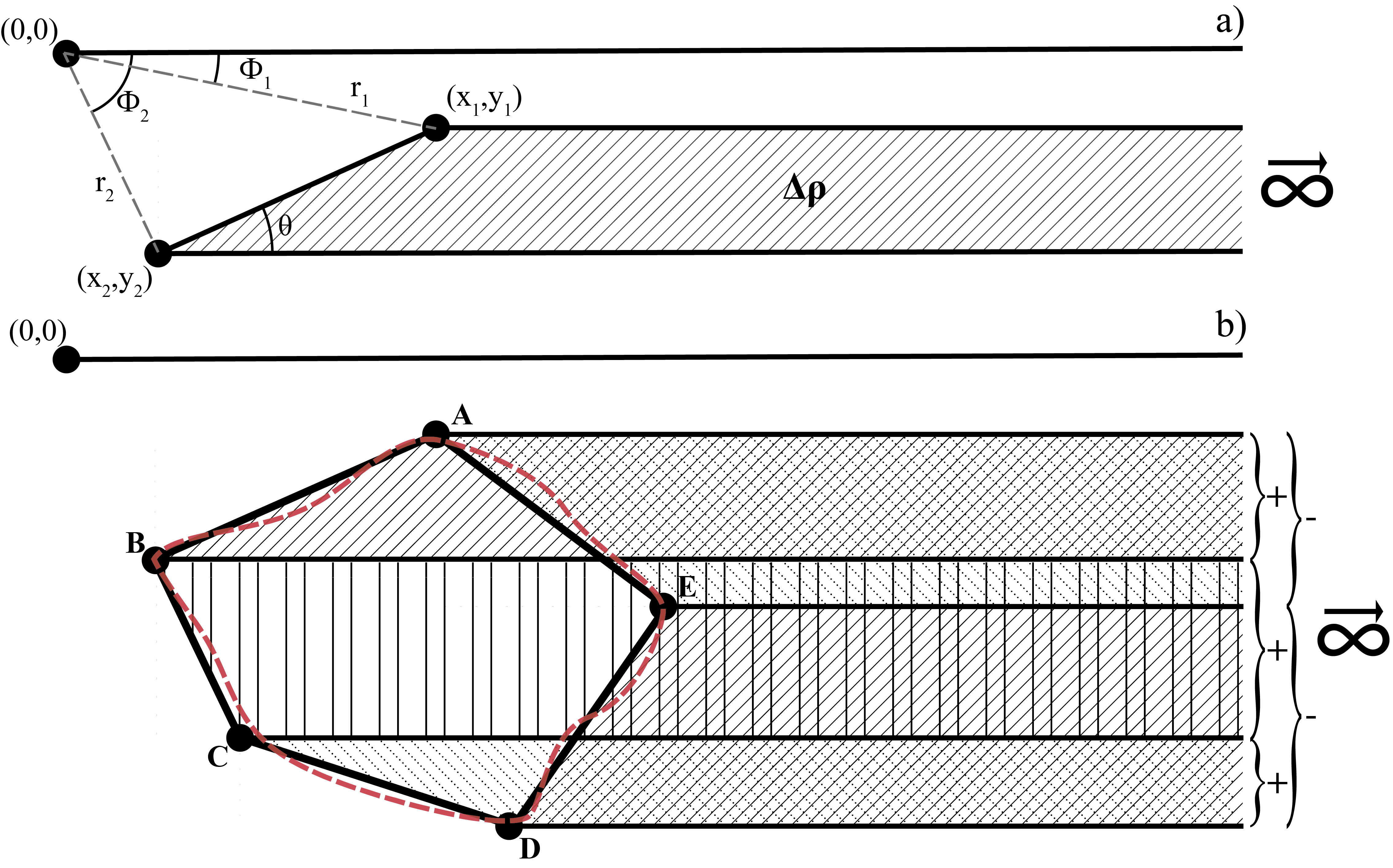
Figure 1 a) An example of a infinite slab with one sloping horizontal side, showing the geometric values relative to the observation point (0,0) using in solving Equation (2). b) Example of calculating the gravity anomaly due to a two dimensional body (red dashed line) estimated using five nodes (A-E) by summing the effects of the five infinite slabs with sloping sides (modified after, Kearey et al., (2013) [5]).

Bott (1969) algorithm testing

To assess the accuracy of the Bott (1969) [1] method, the gravity anomaly determined using the algorithm is compared to that of an exact analytic solution for a simple body. In this case, the solution for a buried horizontal cylinder of constant density contrast, that extends infinitely into and out of the model plane is used. The solution for this case is given by, for example, Garland (1965) [3] Pg. 70 as:

(3)\[g_{z} = 2 \pi G r^{2} \Delta\rho \hspace{2pt} \frac{z}{x^{2}+z^{2}}\]

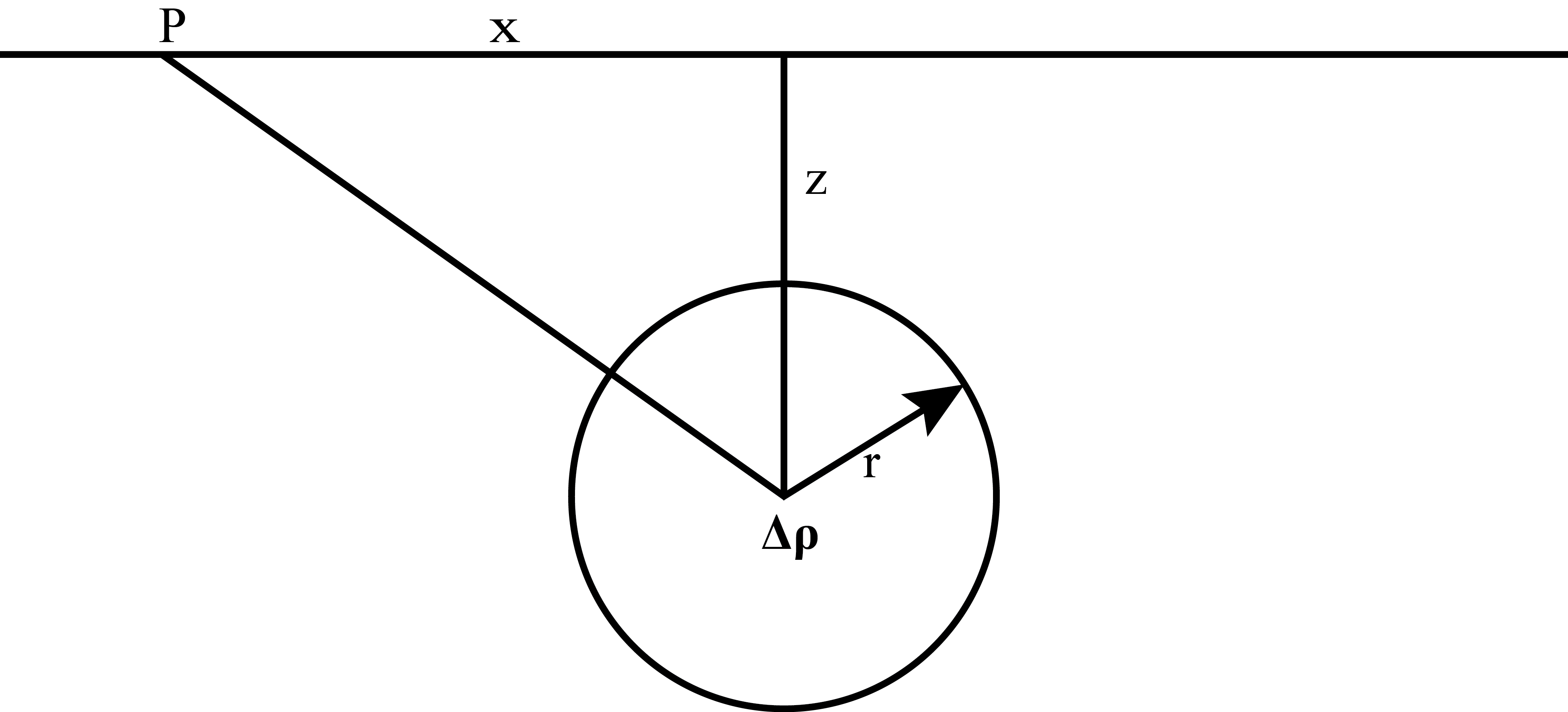
Figure 2 Two-dimensional geometric parameters required for calculating the gravity anomaly produced by a buried cylinder.

Where \(G\) is the Universal Gravitational Constant; \(r\) is the radius of the cylinder; \(\Delta\rho\) is the density contrast between the cylinder and the surrounding material; and \(x\) and \(z\) are the horizontal and vertical distances from the observation point, \(P\), to the centre axis of the cylinder respectively. The geometry of this parametrisation is shown in Figure 2.

Using the Bott (1969) [1] algorithm, the cylinder must be estimated using a series of discrete nodal points, \(N\). A range of values for \(N\) were tested, starting from \(N = 360\) (i.e., one node every 1 degree) and then halving the number of nodes for each new test until \(N = 22\) (i.e., one node every \(\sim\) 16 degrees). For the \(N = 360\) case, the predicted anomaly is also calculated using the Talwani et al., (1959) [10] method for comparison. This method uses a slightly different trigonometric parametrisation.

As can be seen in Figure 3, both the Bott (1969) [1] and Talwani et al., (1959) [10] methods produce almost identical anomalies, with the slight ( \(2.9 \times 10^{-6}\) ) mismatch resulting from the difference between the sum of precision error, due to the different trigonometric functions that are solved by each algorithm. When \(N = 360\), both methods reproduce the analytic anomaly to within an RMS misfit \(9.0 \times 10^{-4}\) mGal. For the \(N = 22\) case the Bott (1969) [1] method predicts the analytic solution to within 0.25 mGal. This level of accuracy is adequate for modelling large scale features, for example, sedimentary basins and lithospheric gravity anomalies and demonstrates that bodies constructed using simplified geometries with relatively few nodes, are sufficient for modelling of such features. However, for some applications, such as microgravity surveys, much higher accuracy is required and detailed polygons with many nodes may be necessary.

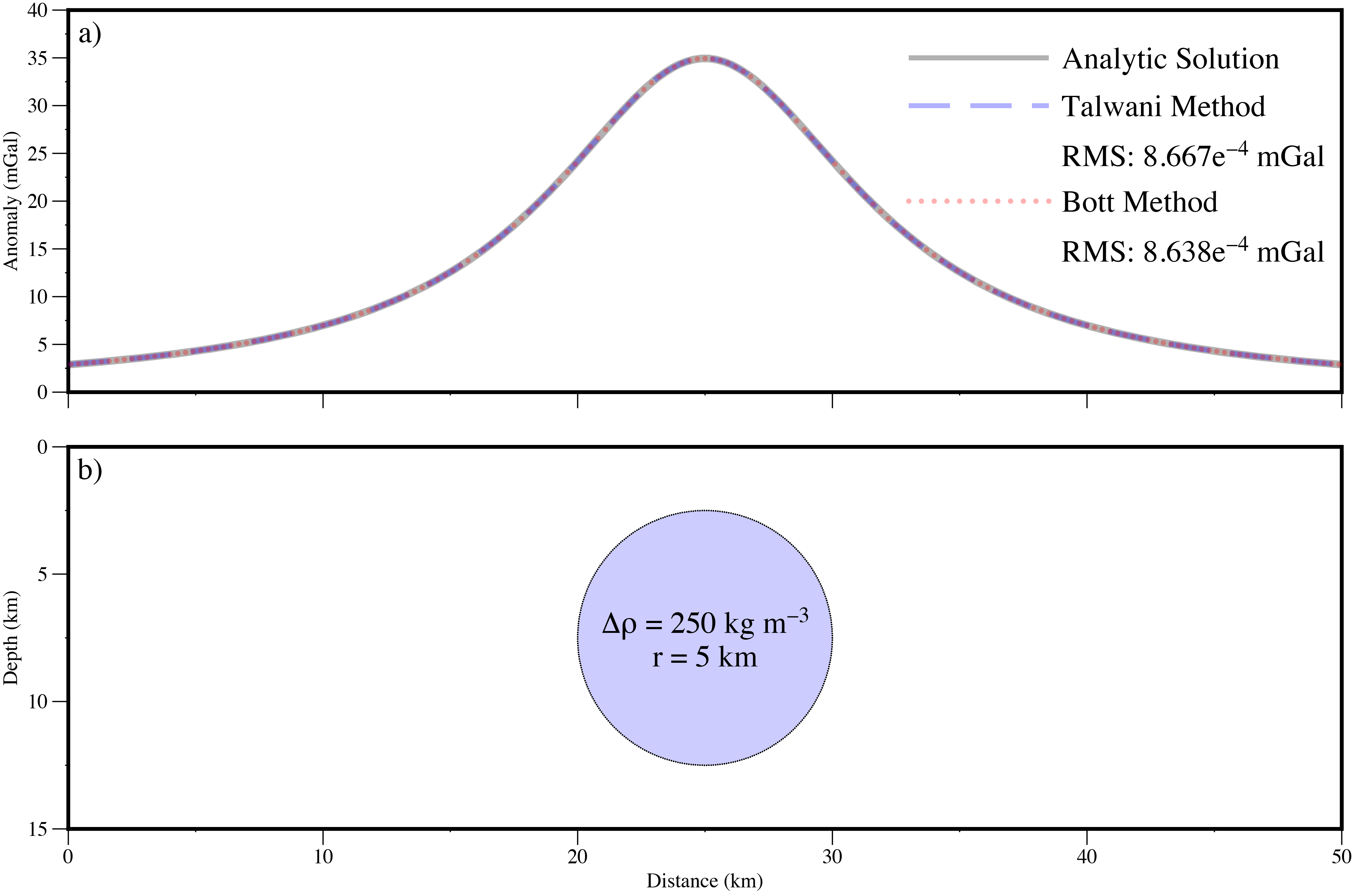
Figure 3 a) Gravity anomaly calculated for the cylinder shown in (b) using an exact analytical solution and by the line-integral methods of Talwani et al., (1959) [10] and Bott (1969) [1]. b) Model cylinder defined using 360 nodes, a radius of 5 \(km\) and a density contrast of \(250\) kg \(m^{-3}\).