A2 Talwani and Heirtzler (1964) magnetic algorithm

Magnetic anomalies are calculated using a python implementation of Talwani and Heirtzler’s (1964) [9] algorithm for two-dimensional uniformly magnetised bodies. This employs a similar procedure to that described in Section A1 for calculating two-dimensional gravity anomalies by treating a body as an n-sided polygon, solving the anomaly for each side and summing the result. However, in the case of magnetic anomalies, there is added complexity owing to the fact that a given bodies magnetisation vector is, for the case of induced magnetisation, dependent on the inclination, delineation and magnitude of the inducing magnetic field (i.e., Earth’s magnetic field). Moreover, if the body has retained a remanent magnetisation, then the magnetisation vector may vary from that of the local Earth field. Furthermore, for two-dimensional modelling, the relationship between the model profile azimuth and the magnetisation vector must also be considered.

These complexities are handled by considering the vertical and horizontal components of the total magnetisation vector separately and then summing these components at the final calculation step. Following the trigonometric parametrisation for a two-dimensional body shown in Figure 4, Talwani and Heirtzler (1964) [9] showed that the horizontal and vertical components of the total magnetic field are given by:

(4)\[V = 2(J_{x}Q - J_{z}P)\]

(5)\[H = 2(J_{x}Q + J_{z}P)\]

where:

(6)\[P = \frac{z_{21}^2}{z_{21}^2+x_{12}^2}(\theta_{1}-\theta_{2}) + \frac{z_{21}x_{12}}{z_{21}^2+x_{12}^2} \log \frac{r_{2}}{r_1}\]

(7)\[Q = \frac{z_{21}x_{12}}{z_{21}^2+x_{12}^2}(\theta_{1}-\theta_{2}) - \frac{z_{21}^2}{z_{21}^2+x_{12}^2} \log \frac{r_{2}}{r_1}\]

and:

(8)\[x_{12}=x_{1}-{x_2} \qquad z_{21}=z_{2}-z_{1} \qquad z_{1}=\sqrt{x_{1}^2+z_{1}^2} \qquad z_{2}=\sqrt{x_{2}^2+z_{2}^2}\]

To account for the bodies magnetisation vector and its relationship with the model profile azimuth \(J_{x}\) and \(J_{z}\) are then given by:

(9)\[J_{x} = J \cos A \cos(C-B)\]

(10)\[J_{z} = J \sin A\]

where angle A is measured in the vertical plane from zero at the horizontal and positive downwards. Angles B and C are measured in the horizontal plane, in a positive clockwise direction from geographic north, as shown in Figure 5.

For the case when magnetisation is induced only:

(11)\[J = kH\]

where \(k\) is the susceptibility contrast between the body and surrounding material and \(H\) is the strength of inducing field. Also, A will be equal to the inclination (I) and B will be equal to the declination (D) of Earth’s field Talwani and Heirtzler (1964) [9].

For the case when magnetisation is remanent or a combination of remanent and induced, the angles A and B will require modification by the user to account for the difference between the inducing field vector and remanent field vector.

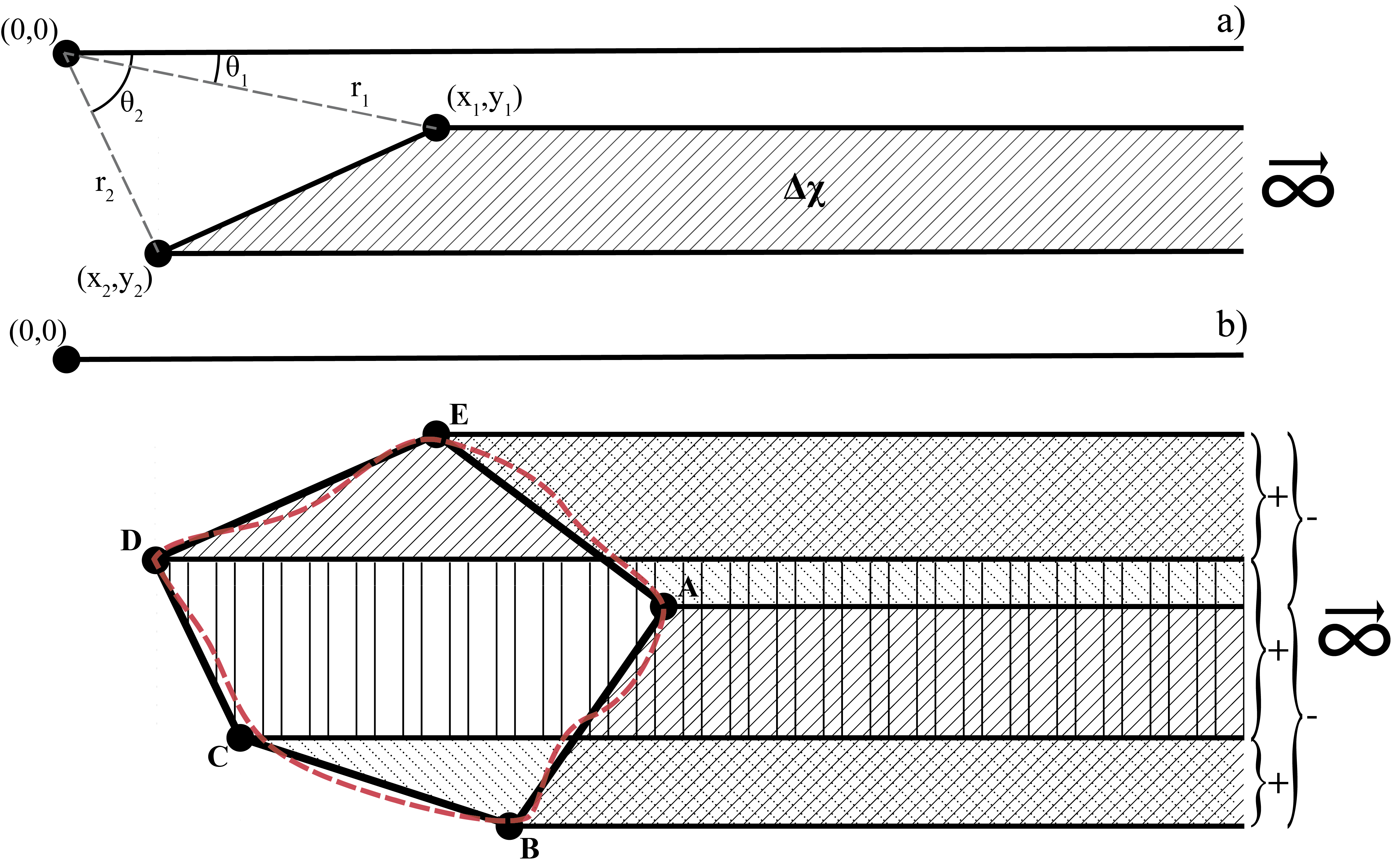
Figure 4 a) Geometric parameters used for solving for the magnetic anomaly produced by an infinite body with one sloping interface. b) Diagram showing an example two-dimensional body (red dashed line) estimated using five nodal points (A-E) (modified after, Talwani and Heirtzler (1964) [9]).

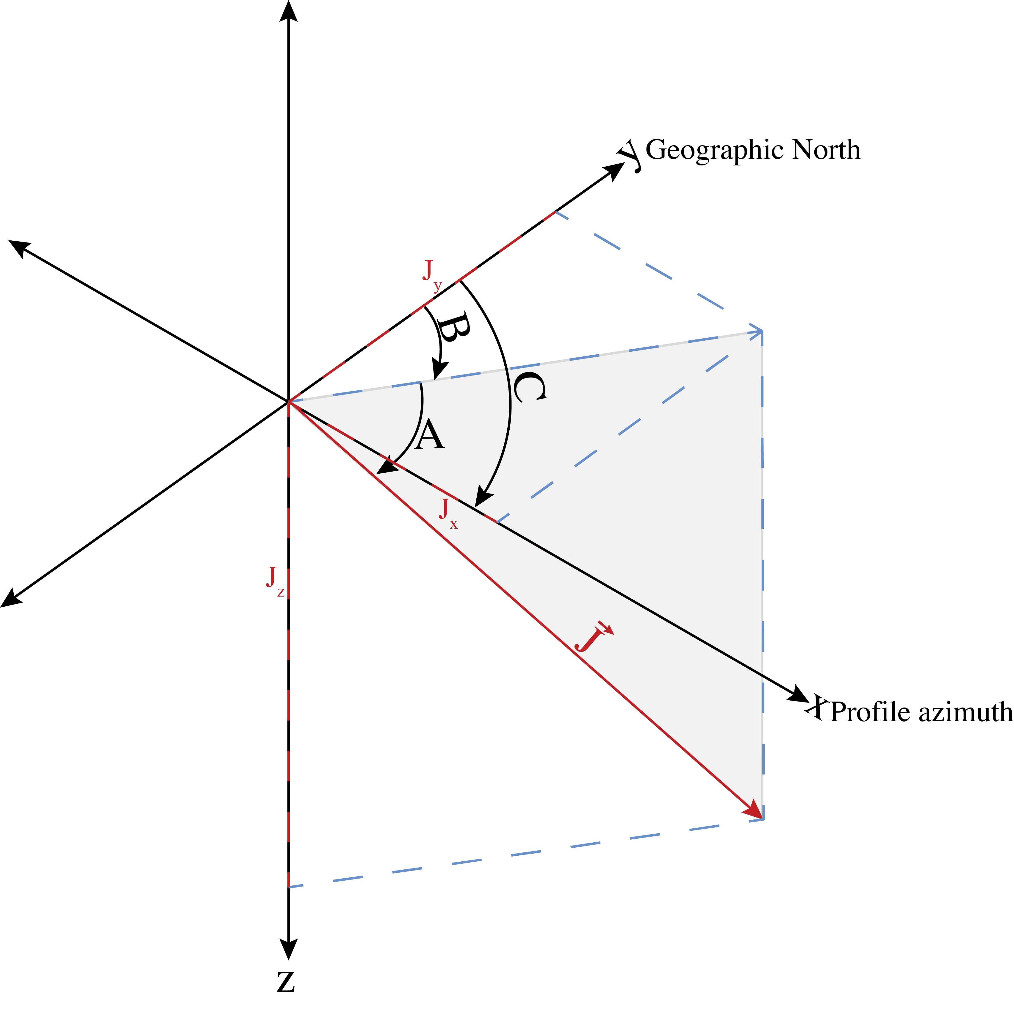
Figure 5 Perspective three-dimensional view of the total magnetisation vector \(\vec{J}\). Grey shade is a vertical plane connecting \(\vec{J}\) to the horizontal x-y surface. A is the dip angle of \(\vec{J}\), measured in the vertical plane and equal to the inclination for induced magnetisation. B and C are the angles between geographic north and the horizontal projection of \(\vec{J}\) and model profile (positive x-axis) respectively. These are measured clockwise from geographic north and B is equal to declination for induced magnetisation (modified after, Talwani and Heirtzler (1964) [9]).

The total magnetic anomaly is then given as the sum of the horizontal and vertical components in the model plane:

(12)\[T = V \sin A + H \cos A \cos (C-B)\]

Talwani and Heirtzler (1964) method testing

To assess the accuracy of the Talwani and Heirtzler (1964) [9] method, the magnetic anomaly determined using the algorithm is compared to that of an exact analytic solution for a simple body. In this case, the solution for a thin (width \(<<\) depth) flat topped vertical sheet with a constant dip angle and magnetisation, which extends infinitely into and out of the model plane and infinitely in depth is solved. The solution for this case is given by, for example, Reford (1964) [7] as:

(13)\[\Delta T = 2kTb^{2}w \left[ \frac{h}{R^{2}} \sin (2I-d) - \frac{x}{R^{2}} \cos(2I-d) \right]\]

(14)\[b^{2} = 1 - \cos{^2}i\sin{^2}D\]

(15)\[I = tan^{-1}[ tan(i) cos(D) ]\]

Where \(k\) is the magnetic susceptibility contrast between the sheet and its surroundings; \(T\) is the strength of the inducing field; \(w\) is the width of the flat top of the sheet; \(h\) is the depth to the top of the dyke; \(i\) is the angle of inclination measured downwards from the horizontal; \(I\) is the angle of inclination of the component of i in the model plane; \(D\) is the angle between magnetic north and the positive x axis (model profile azimuth); \(d\) is the dip of the dyke measured clockwise from the positive x axis (e.g. Figure 5).

This solution is used to simulate a vertical dyke of finite depth extent by calculating the anomalies produced by two bodies, one where \(h=d_{1}\) (the top of the dyke) and a second where \(h = d_{2}\) (the base of the dyke). The effect of the second dyke is subtracted from the first to leave the anomaly caused by a dyke of finite depth extent \(d_{2}\).

Figure 6 shows anomalies calculated using the analytic solution and the Talwani and Heirtzler (1964) [9] algorithm for a thin vertical sheet beginning at a depth of 1 \(km\) and extending to 10 \(km\) with no dip and a magnetic susceptibility of 0.001. Inclination and declination are both 0 degree, and the model azimuth is due north, such that, the sheet strikes east-west.

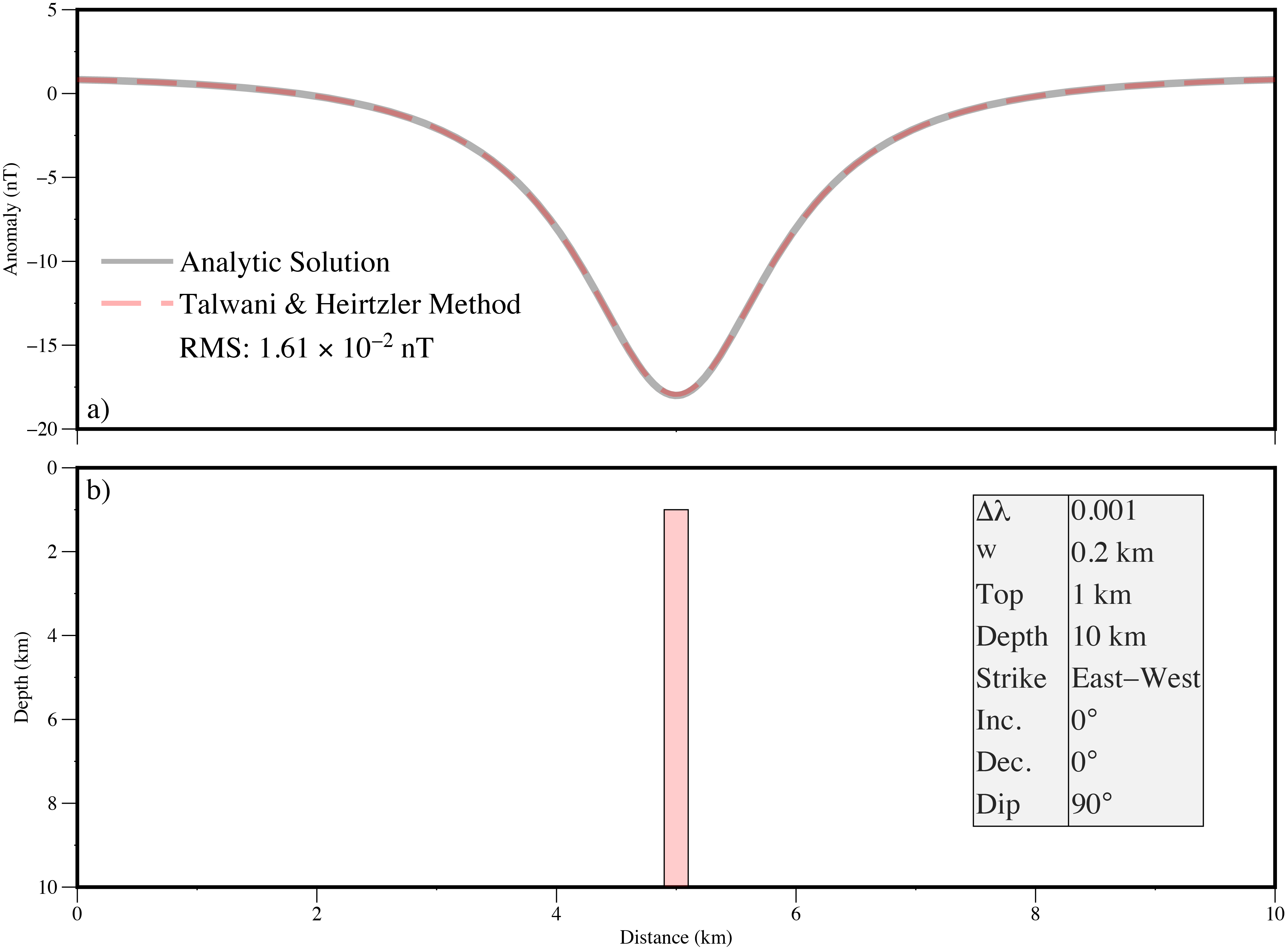
Figure 6 a) Predicted magnetic anomalies for the model shown in (b) using the analytic solution for a thin sheet (grey line) and the Talwani and Heirtzler (1964) [9] algorithm (red dashed line). b) Simple thin sheet model polygon used to simulate a vertical dyke. Inset table lists model parameters (\(\Delta \lambda\)) susceptibility contrast; \(w =\) width of the flat top of the sheet; Inc. and Dec. \(=\) Inclination and Declination of inducing field. Inducing field strength is set as \(50000\) \(nT\). The profile azimuth is east-west.