1.0 Introduction
The purpose of this tutorial is to help familiarise the user with the main features of GMG. It will guide you step-by-step through the process of importing and modeling an example dataset.
We will be working with data related to the Weardale granite, which is located in the Northern Pennines of North England (see Figure 7). Our goal is model the subsurface structure of this granite body and we will use the Bouguer gravity anomaly as our primary dataset. We will thereby recreate the study conducted by British geophysicist Martin Bott in 1967 [2]. In addition to the gravity anomaly, we will also use other supporting datasets including the magnetic anomaly, a borehole record, geological information, and a fictional depth migrated seismic reflection horizon. These auxiliary datasets will help us better constrain the subsurface model and demonstrate how they can be integrated within the GMG modeling environment.
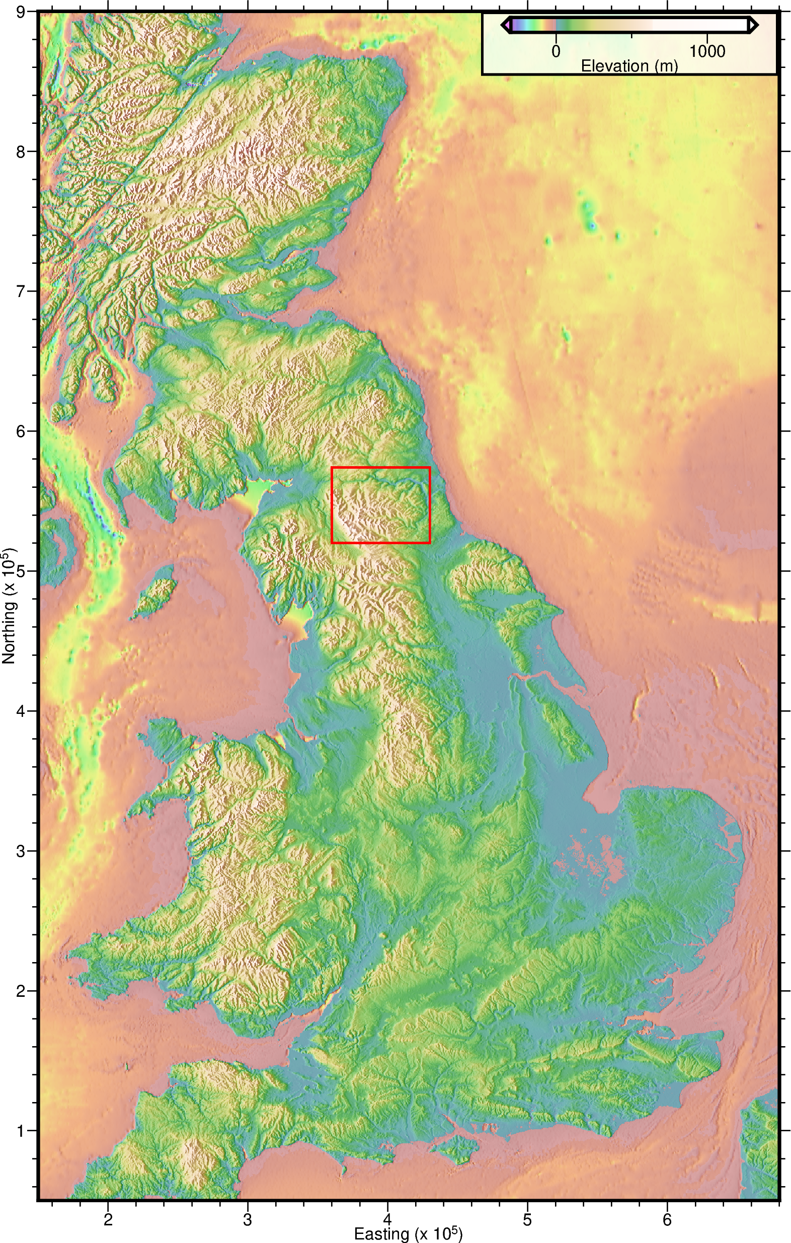
Figure 7 Surface elevation of England showing the location (red box) of our example study region, the Northern Pennines. Note map coordinates are British National Grid Projection [EPSG code: 27700].
The tutorial will guide you through the following steps:
1.  Launching GMG and creating a new 2D model.

2.  Saving the model and reloading it for future use.

3.  Importing observed 2D profile data, including gravity and magnetic anomalies, into the GMG modeling environment.

4.  Incorporating borehole horizon tops into your model.

5.  Adding new layers to your model and assigning attributes such as bulk density and magnetic susceptibility.

6.  Configuring magnetic field attributes in your model, such as the strength of Earth's
    field and the elevation of data acquisition.

7.  Importing XY data points, specifically representing a 2D seismic reflection horizon, into your model.

8.  Running forward model calculations to predict gravity, vertical gravity gradient, and magnetic anomalies.

9.  Using the GMG interface to conduct forward modeling of gravity and magnetic anomalies.

10. Saving the predicted anomaly profiles as external text files.

11. Generating raster figures within GMG's built-in figure production module and saving them to disk.
1.1 Geologic background and potential field datasets
The Weardale granite is situated in the Northern Pennines of Northern England (refer to Figure 7). The existence of this Caledonian-aged granite was initially proposed by Dunham (1934) to explain the observed lead-zinc mineralization in nearby outcrops. Subsequent gravity and magnetic surveys conducted by various researchers strongly supported this hypothesis, and Bott (1967) [2] compiled and published regional maps displaying these data (see Figure 8 and Figure 9). The presence of the granite was finally confirmed through the drilling of the Rookhope borehole by Dunham et al. (1961). The location of this borehole denoted by a yellow circle in Figure 8 and Figure 9.
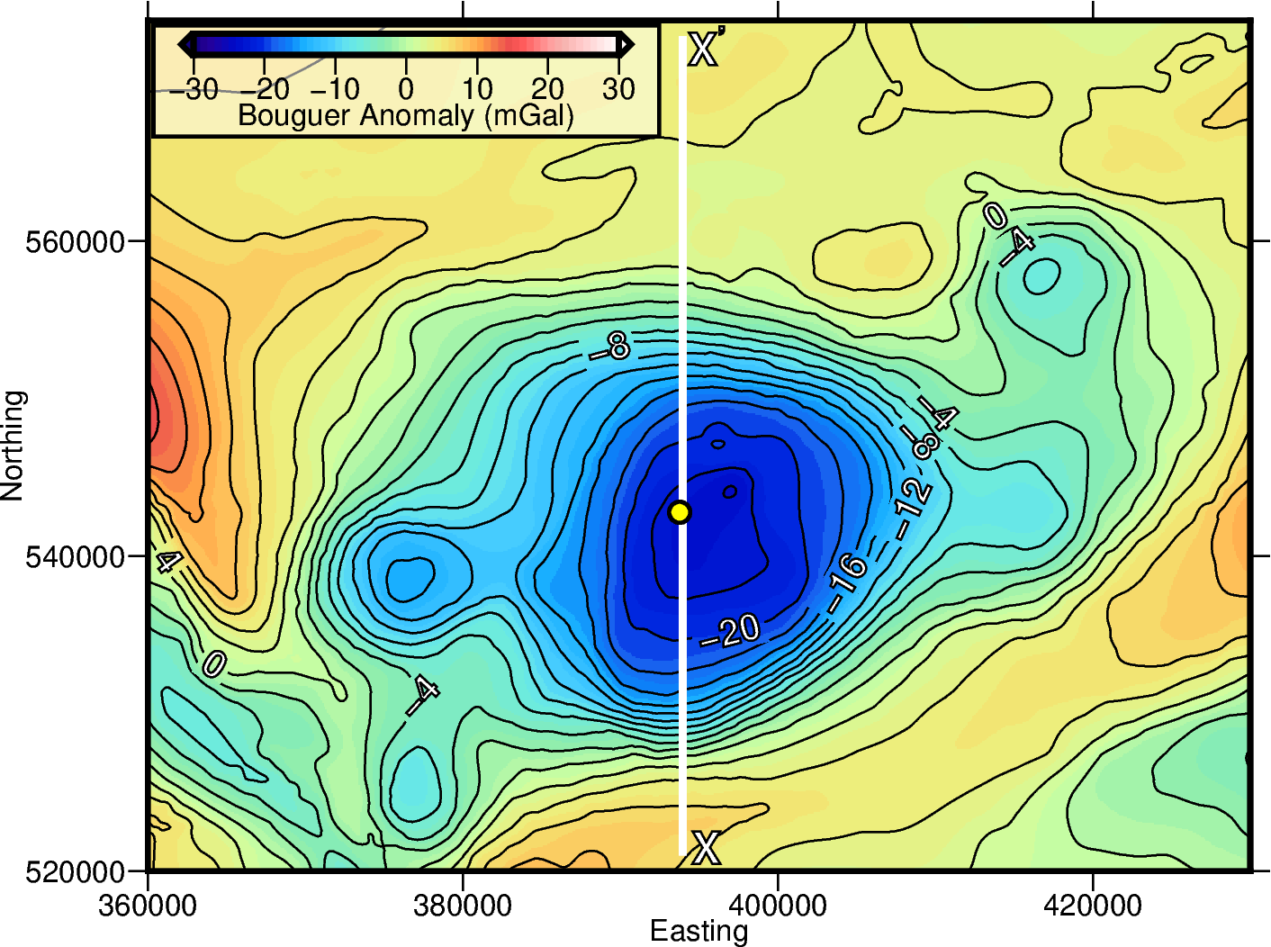
Figure 8 Bouguer gravity anomaly contoured at 2 mGal increments (digitized from figure 2 of Bott (1967) [2]). The white line X-X’ shows the profile we will model in this tutorial. This is chosen to intersect the Rookhope borehole (yellow circle). Note map coordinates are British National Grid Projection [EPSG code: 27700].
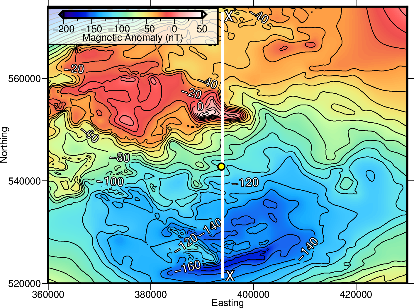
Figure 9 Areo-magnetic anomaly map acquired at an average elevation of 305 m above the ground surface. This survey was flown with a line spacing of 2 km and is contoured at 10 nT increments. The white line X-X’ shows the profile we will model in this tutorial. This is chosen to intersect the Rookhope borehole (yellow circle). Note map coordinates are British National Grid Projection [EPSG code: 27700].