2.0 Pre-modelling data processing and considerations
As we are interested in modelling the structure of the Weardale granite, there are some important pre-modelling steps that we need to consider prior to forward modelling the gravity and magnetic anomalies. These relate to how we deal with other factors (other than the granite) that are contributing to the observed total field anomalies.
A preprocessing step that is commonly applied when focused on modelling near-surface structure is the separation of the “regional” component of the anomaly from the total anomaly. This separation aims to eliminate the contribution from the longer wavelength, regional signal, which may originate from, for example, the juxtaposition of different basement terranes. Typically, regional anomalies produced by deep sources produce much longer wavelength anomalies compared to those associated with near-surface features.
By performing a regional-residual separation, we can focus specifically on the anomalies produced by our target structure. This will aid in generating a more accurate model.
2.1 Gravity anomaly: regional/residual separation
There are several different strategies for calculating regional anomalies. In this case, we will use the regional gravity field as determined by [6] as shown in Figure 10. As can be seen in this figure, there is a long wavelength positive anomaly in this region with amplitudes ranging \(\sim\) \(14-21\) \(mGal\).
We will simply subtract this long wavelength component from the total anomaly, to produce the residual Bouguer anomaly as shown in Figure 11. We will model this residual signal to estimate the subsurface structure of the Weardale granite.
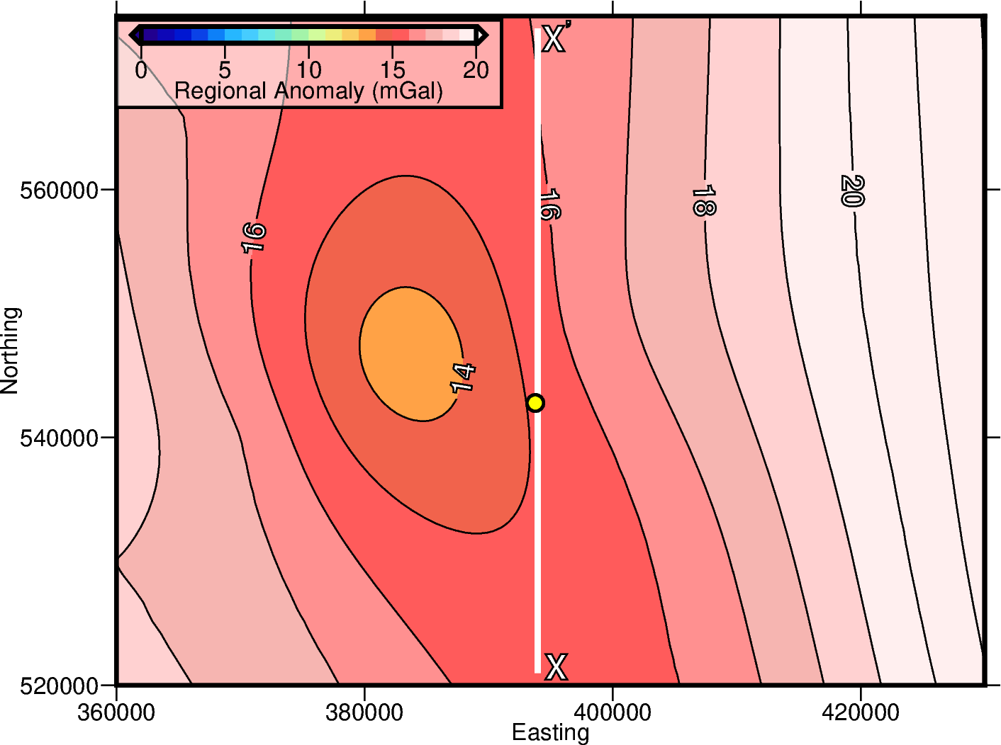
Figure 10 Regional gravity anomaly related to long wavelength density anomalies (as published by [6]). Note, the regional felid is positive, whereas the Waredale granite is expected to produce a negative anomaly relative to the surrounding basement rock.
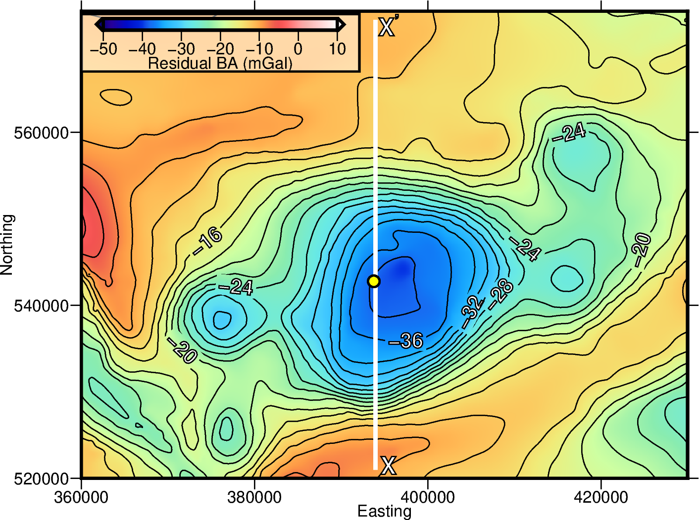
Figure 11 Residual gravity anomaly derived by subtracting the regional anomaly from the total. This reflects the anomaly caused by upper crustal features (i.e., the Weardale granite). Note, the central low (related to the granite) now has a larger amplitude.
2.2 Magnetic anomaly: Reduction To the Pole
In order to model the magnetic anomaly, we’ll apply a Reduction To the Pole (RTP) operation on the grid. We do this to simplify the interpretation of the anomaly as the resulting anomaly appears as if it were observed at the geomagnetic pole, such that, the subsurface bodies are magnetized vertically. This removes the skewness introduced to the observed anomaly as observation latitude decreases. Here, we assume the magnetic sources share the same inclination and declination as the Earth field.
Note
Processing of the magnetic anomaly data was conducted using the python implementation of the Generic Mapping Tools PyGMT. For those interested readers, the Jupyter Notebook containing the processing recipe can be found in the docs/ directory.
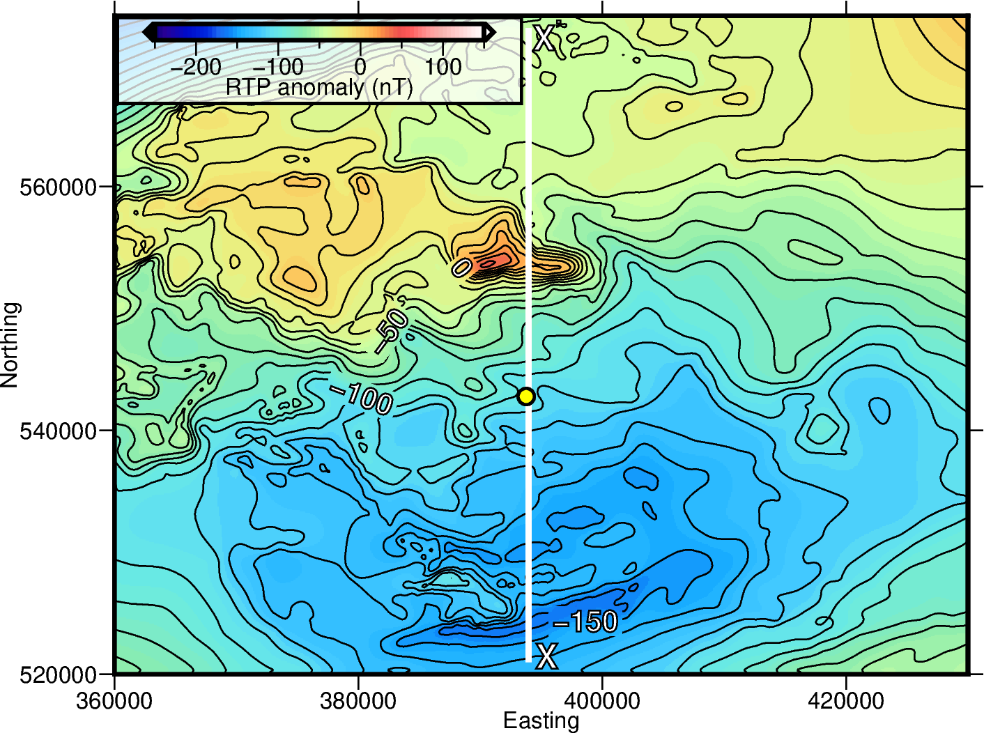
Figure 12 Reduced To Pole magnetic anomaly. The reduction is calculated using the 1964 (when the survey was acquired) inclination and declination of \(9.1\) degrees, and a magnetic declination of \(68.6\) degrees.
2.3 Regional/Residual Separation
Similarly to the gravity grid, we will also perform a regional-residual separation to extract a long wavelength regional field. We then remove regional field from the total field to produce a residual anomaly that reflects near surface sources.
To produce the regional grid we will apply a 2000 m upward continuation operation on the anomaly to transfer the observation elevation from 305 m (the aeromagnetic survey flight height) to 2305 m. This attenuates short wavelengths signals (generated by relatively shallower sources), with the longer wavelength regional field remaining.
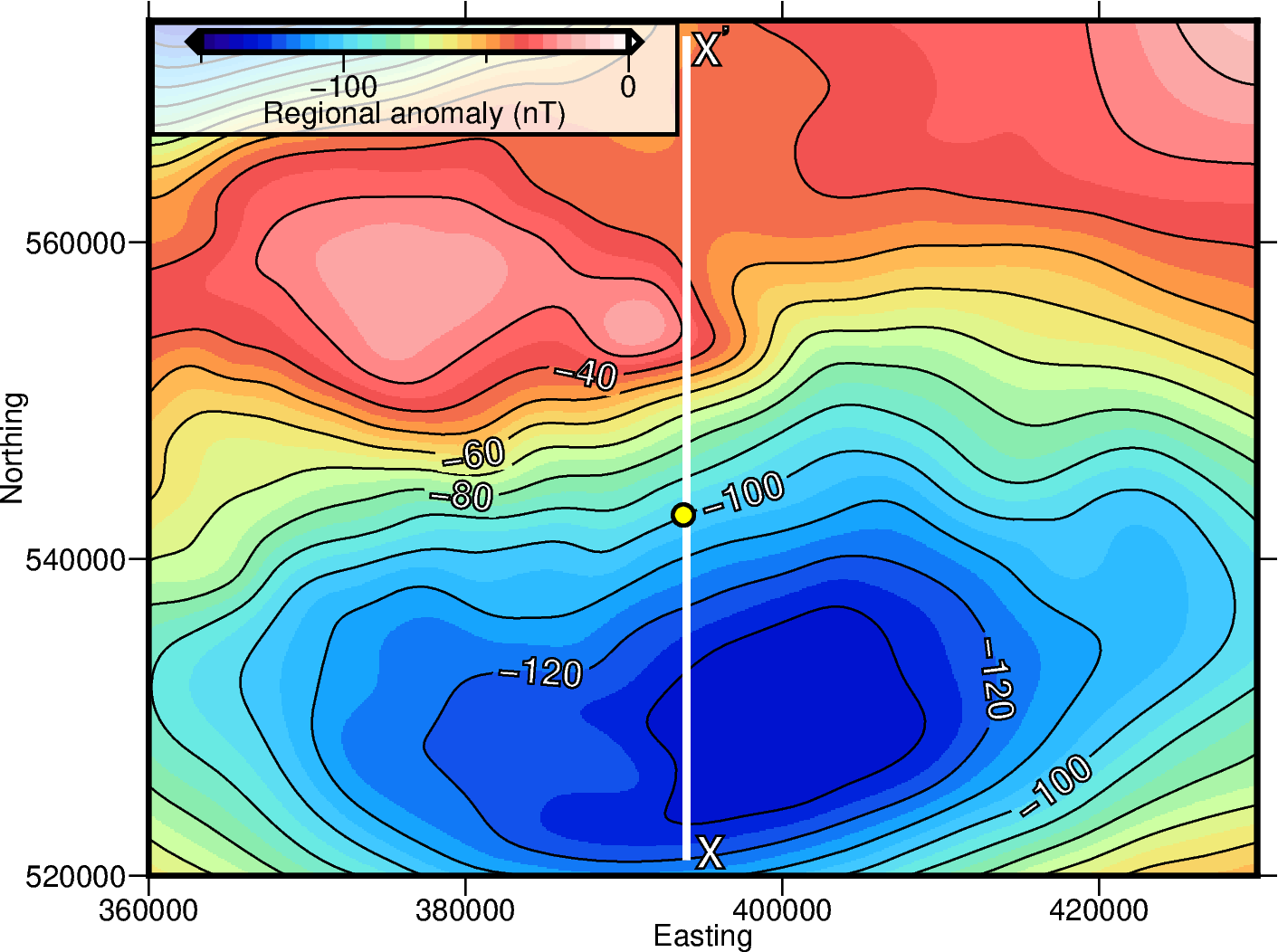
Figure 13 Regional magnetic anomaly derived by upward continuing the observed anomaly to 2700 m.
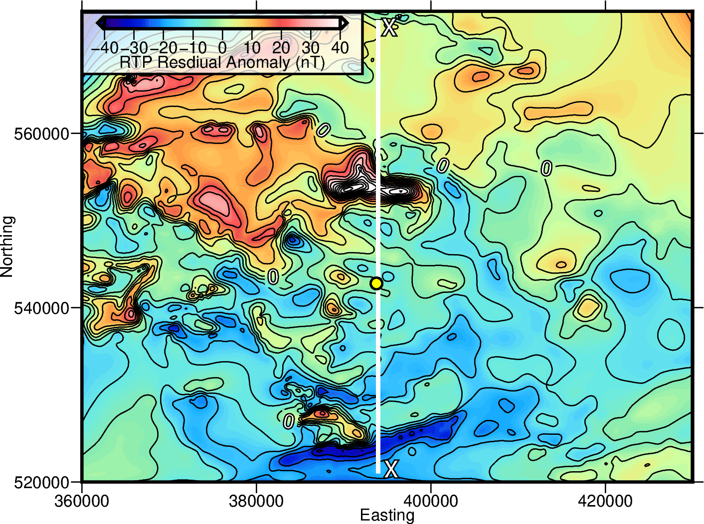
Figure 14 Residual RTP anomaly derived by subtracting the regional anomaly from the Reduced To Pole anomaly. Note, this grid reveals many linear anomalies, related to fault traces, mineral veins, dykes and sills ([6]).